
by Eric · Published · Updated
Bạn đang đọc: A Guide to Conducting Cointegration Tests – Aptech
Introduction
Cointegration is an important tool for modeling the long-run relationships in time series data. If you work with time series data, you will likely find yourself needing to use cointegration at some point.
This blog provides an in-depth introduction to cointegration and will cover all the nuts and bolts you need to get started. In particular, we will look at:
- The fundamentals of cointegration.
- The error correction model.
- How to prepare for cointegration testing.
- What cointegration tests to use with and without structural breaks.
- How to interpret cointegration tests.
- How to perform cointegration tests in GAUSS.
Though not necessary, you may find it helpful to review the blogs on time series modeling and unit root testing before continuing with this blog.
What is Cointegration?
Economic theory suggests that many time series datasets will move together, fluctuating around a long-run equilibrium. In econometrics and statistics, this long-run equilibrium is tested and measured using the concept of cointegration.
Cointegration occurs when two or more nonstationary time series:
- Have a long-run equilibrium.
- Move together in such a way that their linear combination results in a stationary time series.
- Share an underlying common stochastic trend.
What is an Example of Cointegrated Time Series?
Field Supporting Theory Time Series Economics The permanent income hypothesis describes how agents spread their consumption out over their lifetime based on their expected income. Consumption and income. Economics Purchasing power parity is a theory that relates the prices of a basket of goods across different countries. Nominal exchange rates and domestic and foreign prices. Finance The present value model of stock prices implies a long-run relationship between stock prices and their dividends or earnings. Stock prices and stock dividends/earnings. Epidemiology Joint mortality models imply a long-run relationship between mortality rates across different demographics. Male and female mortality rates. Medicine Time series methodologies have been used to examine comorbidities of different types of cancers and trends in medical welfare. Occurrence rates of different types of cancer.
The Mathematics of Cointegration
To understand the mathematics of cointegration, let’s consider a group of time series, $Y_t$, which is composed of three separate time series:
$$y_1 = (y_{11}, y_{12}, ldots, y_{1t})$$ $$y_2 = (y_{21}, y_{22}, ldots, y_{2t})$$ $$y_3 = (y_{31}, y_{32}, …, y_{3t})$$
All three series are nonstationary time series.
Cointegration implies that while $y_1$, $y_2$, and $y_3$ are independently nonstationary, they can be combined in a way that their linear combination is stationary :
$$beta Y_t = beta_1 y_{1t} + beta_2 y_{2t} + beta_3 y_{3t} sim I(0)$$
The Cointegrating Vector In the context of cointegration, $beta$ is commonly known as the cointegrating vector. This vector:
- Dictates how cointegrating series are combined.
- Does not have to be unique – there can be multiple ways of cointegrating.
Normalization Because there can be multiple cointegrating vectors that fit the same economic model, we must impose identification restrictions to normalize the cointegrating vector for estimation.
A common normalization of the cointegrating vector is to set $beta = ( 1, -beta_2, ldots, -beta_N)$. For example, applying these restrictions to our earlier system yields
$$beta Y_t = y_{1t} – beta_2 y_{2t} – beta_3 y_{3t} sim I(0)$$
Part of the appeal of this normalization is that it can be rewritten in a standard regression form
$$y_{1t} = beta_2 y_{2t} + beta_3 y_{3t} + u_t$$
where $u_t$ is a stationary cointegrating error component. Intuitively, $u_t$ can be thought of as short-term deviations from the long-run equilibrium.
While the regression format is a common normalization, it is important to remember that economic theory should inform our identifying restrictions.
What is the Error Correction Model?
Cointegration implies that time series will be connecting through an error correction model. The error correction model is important in time series analysis because it allows us to better understand long-run dynamics. Additionally, failing to properly model cointegrated variables can result in biased estimates.
The error correction model:
- Reflects the long-run equilibrium relationships of variables.
- Includes a short-run dynamic adjustment mechanism that describes how variables adjust when they are out of equilibrium.
- Uses adjustment coefficients to measure the forces that push the relationship towards long-run equilibrium.
The Mathematics of the Error Correction Model
Let’s assume that there is a bivariate cointegrated system with $Y_t = (y_{1t}, y_{2t})$ and a cointegrating vector $beta = (1, -beta_2)$ such that
$$beta Y_{t} = y_{1t} – beta_2 y_{2t}$$
The error correction model depicts the dynamics of a variable as a function of the deviations from long-run equilibrium
$$Delta y_{1t} = c_1 + alpha_1 (y_{1,t-1} – beta_2 y_{2,t-1}) + sum_j psi^j_{11} Delta y_{1, t-j} + sum_j psi^j_{12} Delta y_{2, t-j} + epsilon_1t$$ $$Delta y_{2t} = c_2 + alpha_2 (y_{1,t-1} – beta_2 y_{2,t-1}) + sum_j psi^j_{21} Delta y_{1, t-j} + sum_j psi^j_{22} Delta y_{2, t-j} + epsilon_2t$$
Term Description Intuition $y_{1,t-1} – beta_2 y_{2,t-1}$ Cointegrated long-run equilibrium Because this is an equilibrium relationship, it plays a role in dynamic paths of both $y_{1t}$ and $y_{2t}$. $alpha_1$, $alpha_2$ Adjustment coefficients Captures the reactions of $y_{1t}$ and $y_{2t}$ to disequilibrium. $sum_j psi^j_{11} Delta y_{1, t-j} + sum_j psi^j_{12} Delta y_{2, t-j}$ Autoregressive distributed lags Captures additional dynamics.
Estimating the Error Correction Model
If the cointegrating vector has been previously estimated, then standard OLS or DOLS can be used to estimate the error correction relationship. In this case:
- The estimate of the cointegrating vector can be treated like a known variable.
- The estimated disequilibrium error can be treated like a known variable.
The ECM relationship can be estimated using OLS, seemingly unrelated regressions (SUR), or maximum likelihood estimation.
The Vector Error Correction Model (VECM)
The vector error correction model (VECM) is the multivariate extension of the ECM. If we are working in a vector autoregressive context, cointegration implies a VECM such that
$$Delta Y_t = Phi D_t + Pi Y_{t-1} + Gamma_1 Delta Y_{t-1} + cdots + Gamma_{p-1} Delta Y_{t-p+1} + epsilon_t$$
Like the ECM, the VECM parameters reflect the long-run and short-run dynamics of system as shown in the table below:
Term Description Intuition $Pi$ Long-run impact matrix. $Pi = Pi_1 + Pi_2 + cdots + Pi_p – I_n$, captures adjustments towards the long-run equilibrium and contains the cointegrating relationships. $Gamma_k$ Short-run impact matrix. The short-run impact matrix is constructed from $-sum_{j=k+1}^p Pi_j$ and captures short-run deviations from the equilibrium. $D_t$ Deterministic terms. These terms take the form $D_t = u_0 + u_1 t$ where $u_0$ is the constant component and $u_1 t$ is the trend component.
Estimating the VECM
The VECM model can be estimated using the Johansen method:
- Estimate the appropriate VAR(p) model for $Y_t$.
- Determine the number of cointegrating vectors, using a likelihood ratio test for the rank of $Pi$.
- Impose identifying restrictions to normalize the cointegrating vector.
- Using the normalized cointegrating vectors, estimate the resulting VECM by maximum likelihood.
Preparing For Cointegration Tests
Before jumping directly to cointegration testing, there are a number of other time series modeling steps that we should consider first.
Establishing Underlying Theory
One of the key considerations prior to testing for cointegration, is whether there is theoretical support for the cointegrating relationship. It is important to remember that cointegration occurs when separate time series share an underlying stochastic trend. The idea of a shared trend should be supported by economic theory.
As an example, consider growth theory which suggests that productivity is a key driver of economic growth. As such, it acts as the common trend, driving the comovements of many indicators of economic growth. Hence, this theory implies that consumption, investment, and income are all cointegrated.
Time Series Visualization
One of the first steps in time series modeling should be data visualization. Time series plots provide good preliminary insights into the behavior of time series data:
- Is a series mean-reverting or has explosive behavior?
- Does it have a time trend?
- Is there seasonality?
- Are there structural breaks?
Unit Root Testing
We’ve established that cointegration occurs between nonstationary, I(1), time series. This implies that before testing for or estimating a cointegrating relationship, we should perform unit root testing.
Our previous blog, “How to Conduct Unit Root Testing in GAUSS”, provides an in-depth look at how to perform unit root testing in GAUSS.
GAUSS tools for performing unit root tests are available in a number of libraries, including the Time Series MT (TSMT), the open-source TSPDLIB, and the coint libraries. All of these can be directly located and installed using the GAUSS package manager.
Full example programs for testing for unit roots using TSMT procedures and TSPDLIB procedures are available on our Aptech GitHub page.
Panel Data Unit Root Test TSMT procedure TSPDLIB procedure Hadri hadri Im, Pesaran, and Shin ips Levin-Lu-Chin llc Schmidt and Perron LM test lm Breitung and Das breitung Cross-sectionally augmented IPS test (CIPS) cips Panel analysis of nonstationary and idiosyncratic and common (PANIC) bng_panic Time Series Unit Root Test TSMT procedure TSPDLIB procedure Augmented-Dickey Fuller vmadfmt adf Phillips-Perron vmppmt pp KPSS kpss lmkpss Schmidt and Perron LM test lm GLS-ADF dfgls dfgls Quantile ADF qr_adf
Testing for structural breaks
A complete time series analysis should consider the possibility that structural breaks have occurred. In the case that structural breaks have occurred, standard tests for cointegration are invalid.
Therefore, it is important to:
- Test whether structural breaks occur in the individual series.
- In the case that there is evidence of structural breaks, employ cointegration tests that allow for structural breaks.
The GAUSS sbreak procedure, available in TSMT, is an easy-to-use tool for identifying multiple, unknown structural breaks.
Cointegration Tests
In order to test for cointegration, we must test that a long-run equilibrium exists for a group of data. There are a number of things that need to be considered:
- Are there multiple cointegrating vectors or just one?
- Is the cointegrating vector known or does it need to be estimated?
- What deterministic components are included in the cointegrating relationship?
- Do we suspect structural breaks in the cointegrating relationship?
In this section, we will show how to use these questions to guide cointegration testing without structural breaks.
The Engle-Granger Cointegration Test
The Engle-Granger cointegration test considers the case that there is a single cointegrating vector. The test follows the very simple intuition that if variables are cointegrated, then the residual of the cointegrating regression should be stationary.
Forming the cointegrating residual How to form the cointegrating residual depends on if the cointegrating vector is known or must be estimated:
If the cointegrating vector is known, the cointegrating residuals are directly computed using $u_t = beta Y_t$. The residuals should be stationary and:
- Any standard unit root tests, such as the ADF or PP test, can be used to test the residuals. The test statistics follow the standard distributions.
- The test compares the null hypothesis of no cointegration against the alternative of cointegration.
- The cointegrating residuals should be examined for the presence of a constant or trend, and the appropriate unit root test should be utilized.
If the cointegrating vector is unknown, OLS is used to estimate the normalized cointegrating vector from the regression $$y_{1t} = c + beta y_{2t} + u_{t}$$
- The residuals from the cointegrating regression are estimated $$hat{u_t} = y_{1t} – hat{c} – hat{beta_2}y_{2t}$$
- Any standard unit root test, such as the ADF or PP test, can be used to test the residuals. The test statistics follow the nonstandard Phillips-Ouliaris (PO) distributions.
- The PO distribution depends on the trend behavior of the data.
The Johansen Tests
There are two Johansen cointegrating tests for the VECM context, the trace test and the maximal eigenvalue test. These tests hinge on the intuition that in the VECM, the rank of the long-run impact matrix, $Pi$, determines if the VAR(p) variables are cointegrated.
Since the rank of the long-run impact matrix equals the number of cointegrating relationships:
- A likelihood ratio statistic for determining the rank of $Pi$ can be used to establish the number of cointegrating relationships.
- Sequential testing can be used to test the number, $k$, of the cointegrating relationships.
The Johansen testing process has two general steps:
- Estimate the VECM model using maximum likelihood under various assumptions:
- With and without trend.
- With and without constant.
- With varying number, $k$, of cointegrating vectors.
- Compare the models using likelihood ratio tests.
The Johansen Trace Statistics The Johansen trace statistic:
- Is a likelihood ratio test of an unrestricted VECM against the restricted VECM with $k$ cointegrating vectors, where $k = m-1, ldots, 0$.
- Is formed from the trace of a diagonal matrix of generalized eigenvalues from $Pi$.
- As the $LR_{trace}(k)$ statistic gets closer to zero, we are less likely to reject the null hypothesis.
- If the $LR_{trace}(k)>CV$, then the null hypothesis is rejected.
The Johansen testing procedure sequentially tests the null hypothesis that the number of cointegrating vectors, $k = m$ against the alternative that $k > m$.
Stage Null Hypothesis Alternative Conclusion One $H_0: k = 0$ $H_A: k>0$ If $H_0$ cannot be rejected, stop testing, and $k = 0$. If null is rejected, perform next test. Two $H_0: k leq 1$ $H_A: k>1$ If $H_0$ cannot be rejected, stop testing, and $k leq 1$. If null is rejected, perform next test. Three $H_0: k leq 2$ $H_A: k>2$ If $H_0$ cannot be rejected, stop testing, and $k leq 2$. If null is rejected, perform next test. m-1 $H_0: k leq m-1$ $H_A: k>m-1$ If $H_0$ cannot be rejected, stop testing, and $k leq m-1$. If null is rejected, perform next test.
The test statistic follows a nonstandard distribution and depends on the dimension and the specified deterministic trend.
The Johansen Maximum Eigenvalue Statistic The maximal eigenvalue statistic:
- Considers the null hypothesis that the cointegrating rank is $k$ against the alternative hypothesis that the cointegrating rank is $k + 1$.
- The statistic follows a nonstandard distribution.
Cointegration Test with Structural Breaks
In the case that there are structural breaks in the cointegrating relationship, the cointegration tests in the previous station should not be used. In this section we look at three tests for cointegration with structural breaks:
- The Gregory and Hansen (1996) test for cointegration with a single structural break.
- The Hatemi-J test (2009) for cointegration with two structural breaks.
- The Maki test for cointegration with multiple structural breaks.
The Gregory and Hansen Cointegration Test
The Gregory and Hansen (1996) cointegration test is a residual-based cointegration test that tests the null hypothesis of no cointegration against the alternative of cointegration in the presence of a single regime shift.
The Gregory and Hansen (1996) test:
- Is an extension of the ADF and PP residual tests for cointegration.
- Allows for unknown regimes shifts in either the intercept or the coefficient vector.
- Is valid for three different model cases: level shift with trend, regime shifts (changes in coefficients), regime shift with a shift in trend.
Because the structural break date is unknown, the test computes the cointegration test statistic for each possible breakpoint, and the smallest test statistics are used.
Gregory and Hansen (1996) suggest running their tests in combination with the standard cointegration tests:
- If the standard ADF test and the Gregory and Hansen ADF test both reject the null hypothesis of no cointegration, there is evidence in support of cointegration.
- If the standard ADF test does not reject the null hypothesis but the Gregory and Hansen ADF does, structural change in the cointegrating vector may be important.
- If the standard ADF test and the Gregory and Hansen ADF both reject the null hypothesis, there is no evidence from this test that structural change has occurred.
The Hatemi-J Cointegration Test with Two Structural Breaks
The Hatemi-J cointegration test is an extension of the Gregory and Hansen cointegration test. It allows for two possible structural breaks with unknown timing.
The Maki Cointegration Test
The Maki cointegration test builds on the Gregory and Hansen and the Hatemi-J cointegration tests to allow for an unknown number of structural breaks.
Where to Find Cointegration Tests for GAUSS
GAUSS tools for performing cointegration tests and estimating VECM models are available in a number of libraries, including the Time Series MT (TSMT) library, TSPDLIB, and the coint libraries. All of these can be directly located and installed using the GAUSS package manager.
Cointegration test Null Hypothesis Decision Rule GAUSS library Engle-Granger (ADF) No cointegration. Reject the null hypothesis if the $ADF$ test statistic is less than the critical value. TSMT, tspdlib, coint Phillips No cointegration. Reject the null hypothesis if the $Z$ test statistic is less than the critical value. coint, tspdlib Stock and Watson common trend $Y$ is a non-cointegrated system after allowing for the pth order polynomial common trend. Reject the null hypothesis if the $SW$ test statistic is less than the critical value. coint Phillips and Ouliaris $Y$ and $X$ are not cointegrated. Reject the null hypothesis if the $P_u$ or $P_z$ statistic is greater than the critical value. coint, tspdlib Johansen trace Rank of $Pi$ is equal to $r$ against the alternative that the rank of $Pi$ is greater than $r$. Reject the null hypothesis if $LM_{max}(k)$ is greater than the critical value. TSMT, coint Johansen maximum eigenvalue Rank of $Pi$ is equal to $r$ against the alternative that the rank of $Pi$ is equal to $r+1$. Reject the null hypothesis if $LM(r)$ is greater than the critical value. TSMT, coint Gregory and Hansen No cointegration against the alternative of cointegration with one structural break. Reject the null hypothesis if $ADF$, $Z_{alpha}$, or $Z_t$ are less than the critical value. tspdlib Hatemi-J No cointegration against the alternative of cointegration with an unknown number of structural breaks. Reject the null hypothesis if $ADF$, $Z_{alpha}$, or $Z_t$ are less than the critical values. tspdlib Maki No cointegration against the alternative of cointegration with two structural breaks. Reject the null hypothesis if $ADF$, $Z_{alpha}$, or $Z_t$ are less than the critical value. tspdlib Shin test Cointegration. Reject the null hypothesis if the test statistic is less than the critical value. tspdlib
How to Test for Cointegration using GAUSS
In this section, we will test for cointegration between monthly gold and silver prices, using historic monthly price date starting in 1915. Specifically, we will work through several stages of analysis:
- Graphing the data and checking deterministic behavior.
- Testing each series for unit roots.
- Testing for cointegration without structural breaks.
- Testing for cointegration with structural breaks.
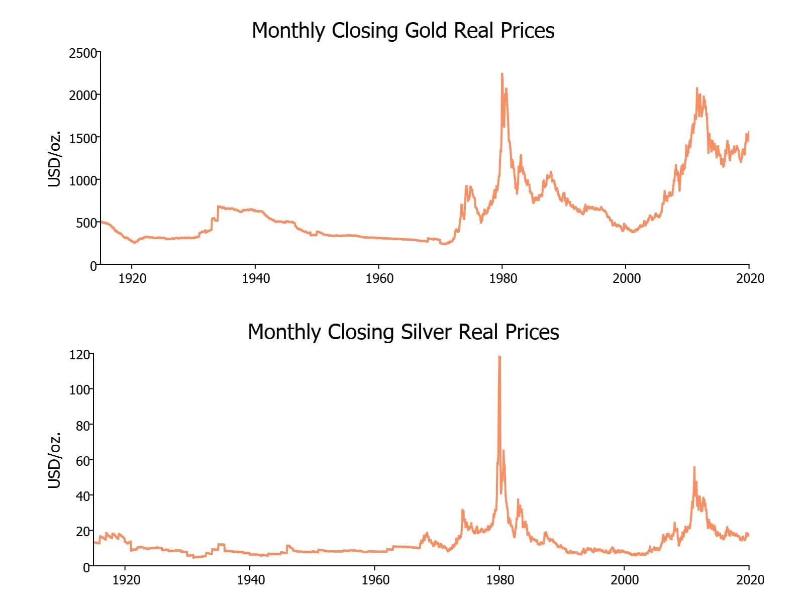
Graphing the Data
As a first step, we will create a time series graph of our data. This allows us to visually examine the deterministic trends in our data.
Tìm hiểu thêm: Thương hiệu cá nhân là gì? Làm sao để xây dựng thương hiệu cá nhân thành công
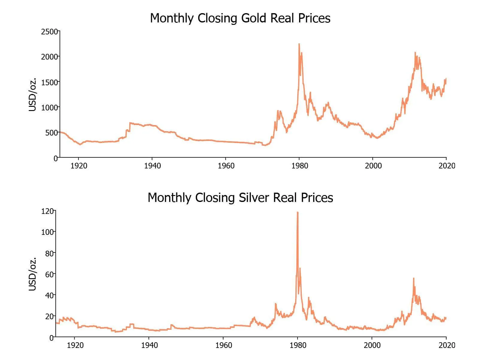
From our graphs, we can draw some preliminary conclusions about the dynamics of gold and silver prices over our time period:
- There appears to be some foundation for the comovement of silver and gold prices.
- Neither gold nor silver prices appear to have a time trend.
Testing Each Series for Unit Roots
Before testing if silver and gold prices are cointegrated, we should test if the series have unit roots. We can do this using the unit roots tests available in the TSMT and TSPDLIB libraries.
Gold monthly closing prices (2015-2020) Time Series Unit Root Test Test Statistic Conclusion Augmented-Dickey Fuller -1.151 Cannot reject the null hypothesis of unit root. Phillips-Perron -1.312 Cannot reject the null hypothesis of unit root. KPSS 2.102 Reject the null hypothesis of stationarity at the 1% level. Schmidt and Perron LM test -2.399 Cannot reject the null hypothesis of unit root. GLS-ADF -0.980 Cannot reject the null hypothesis of unit root. Silver monthly closing prices (2015-2020) Time Series Unit Root Test Test Statistic Conclusion Augmented-Dickey Fuller -5.121 Reject the null hypothesis of unit root at the 1% level. Phillips-Perron -5.446 Reject the null hypothesis of unit root at the 1% level. KPSS 0.856 Reject the null hypothesis of stationarity at the 1% level. Schmidt and Perron LM test -4.729 Reject the null hypothesis of unit root at the 1% level. GLS-ADF -4.895 Reject the null hypothesis of unit root at the 1% level.
These results provide evidence that gold prices are nonstationary but suggest that the silver prices are stationary. At this point, we would not likely proceed with cointegration testing or we may wish to perform additional unit root testing. For example, we may want to perform unit root tests that allow for structural breaks.
The GAUSS code for the tests in this section is available here.
Testing for Cointegration
Now, let’s test for cointegration without structural breaks using two different tests, the Johansen tests and the Engle-Granger test.
The Johansen Tests We will use the vmsjmt procedure from the TSMT library. This procedure should be used with the vmc_sjamt and vmc_sjtmt procedures, which find the critical values for the Maximum Eigenvalue and Trace statistics, respectively.
The vmsjmt procedure requires four inputs:
y Matrix, contains the data to be tested for cointegration. p Scalar, the order of the time polynomial in the fitted regression. Set to $p=-1$ for no deterministic component, $p=0$ for a constant only, $p=1$ for a constant and trend. k Scalar, the number of lagged differences to use when computing the estimator. no_det Scalar, set $no_det = 1$ to suppress the constant term from the fitted regression and include it in the cointegrating regression.
The vmsjmt procedure returns both the Johansen Trace and the Johansen Maximum Eigenvalue statistic. In addition, it returns the associated eigenvalues and eigenvectors.
new; // Load tsmt library library tsmt; // Set filename (with path) for loading fname2 = __FILE_DIR $+ “commodity_mon.dat”; // Load real prices data y_test_real = loadd(fname2, “P_gold_real + P_silver_real”); // No deterministic component // the fitted regression p = -1; // Set number of lagged differences // for computing estimator k = 2; // No determinant no_det = 0; { ev, evec, trace_stat, max_ev } = vmsjmt(y_test_real, p, k, no_det); cv_lr2 = vmc_sjamt(cols(y), p); cv_lr1 = vmc_sjtmt(cols(y), p);
Both trace_stat and max_ev will contain statistics for all possible ranks of $Pi$.
For example, since we are testing for cointegration of just two time series, there will be at most one cointegrating vector. This means trace_stat and max_ev will be 2 x 1 matrices, testing both null hypotheses that $r=0$ and $r=1$.
Test Test Statistic 10% Critical Value Conclusion Johansen Trace Statistic $$H_0: r=1, 56.707$$ $$H_0: r=0, 0.0767$$ 10.46 Cannot reject the null hypothesis that $r=0$. Johansen Maximum Eigenvalue $$H_0: r=1, 56.631$$ $$H_0: r=0, 0.0766$$ 9.39 Cannot reject the null hypothesis that $r=0$.
These results indicate that there is no cointegration between monthly gold and silver prices. This should not be a surprise, given the results of our unit root testing.
The Engle-Granger Since there is only one possible cointegrating vector for this system, we could have also used the Engle-Granger test for cointegration. This test can be implemented using the coint_egranger procedure from the TSPDLIB library.
The coint_egranger procedure requires five inputs:
y Vector, independent variable in the testing regression. This is the variable the cointegrating variable is normalized to. X Matrix, dependent variable(s) in the testing regression. This should contain all other variables. model Scalar, specifies which deterministic components to include in the model. Set equal to 0 to include no deterministic components, 1 to include a constant, and 2 to include a constant and trend. pmax Scalar, the maximum number of lags to include in the cointegrating vector. ic Scalar, which information criteria to use to select the lags included in the ADF regression. Set equal to 1 for the AIC, 2 for the SIC.
The coint_egranger procedure returns the test statistic along with the 1%, 5% and 10% critical values.
Using the data already loaded in the previous example:
/* ** Information Criterion: ** 1=Akaike; ** 2=Schwarz; ** 3=t-stat sign. */ ic = 2; // Maximum number of lags pmax = 12; // No constant or trend model = 0 { tau0, cvADF0 } = coint_egranger(y_test_real[., 1], y_test_real[., 2], model, pmax, ic); // Constant model = 1 { tau1, cvADF1 } = coint_egranger(y_test_real[., 1], y_test_real[., 2], model, pmax, ic); // Constant and trend model = 2 { tau2, cvADF2 } = coint_egranger(y_test_real[., 1], y_test_real[., 2], model, pmax, ic); Test Test Statistic 10% Critical Value Conclusion Engle-Granger, no constant -3.094 -2.450 Reject the null of no cointegration at the 10% level. Engle-Granger, constant -1.609 -3.066 Cannot reject the null hypothesis of no cointegration. Engle-Granger, constant and trend -2.327 -3.518 Cannot reject the null hypothesis of no cointegration.
These results provide evidence for our conclusion that there is no cointegration between gold and silver prices. Note, however, that these results are not conclusive and depend on whether we include a constant. This sheds light on the importance of including the correct deterministic components in our model.
Testing for Cointegration with Structural Breaks
To be thorough we should also test for cointegration using tests that allow for a structural break. As an example, let’s use the Gregory-Hansen test to compare the null hypothesis of no cointegration against the alternative that there is cointegration with one structural break.
This test can be implemented using the coint_ghansen procedure from the TSPDLIB.
The coint_ghansen procedure requires eight inputs:
y Vector, dependent variable in the testing regression. This is the variable the cointegrating variable is normalized to. X Matrix, independent variable(s) in the testing regression. This should contain all other variables. model Scalar, specified what type of regime shifts to include. Set equal to 1 for a level shift (C model), 2 for level shift with trend (C/T model), 3 for regime shift (C/S model), and 4 for regime and trend shifts. bwl Scalar, Bandwidth for kernel estimator for Phillips-Perron type test. pmax Scalar, the maximum number of lags to include in the cointegrating vector. ic Scalar, which information criteria to use to select the lags included in the ADF regression. Set equal to 1 for the AIC, 2 for the SIC. varm Scalar, long-run consistent variance type to use for the Phillips-Perron type test: 1 = iid, 2 = Bartlett, 3 = Quadratic Spectral (QS), 4 = SPC with Bartlett /see (Sul, Phillips & Choi, 2005), 5 = SPC with QS, 6 = Kurozumi with Bartlett, 7 = Kurozumi with QS. trimm Scalar, amount to trim from consideration as break date. /* ** Information Criterion: ** 1=Akaike; ** 2=Schwarz; ** 3=t-stat sign. */ ic = 2; //Maximum number of lags pmax = 12; // Trimming rate trimm= 0.15; // Long-run consistent variance estimation method varm = 3; // Bandwidth for kernel estimator T = rows(y_test_real); bwl = round(4 * (T/100)^(2/9)); // Level shift model = 1; { ADF_min1, TBadf1, Zt_min1, TBzt1, Za_min1, TBza1, cvADFZt1, cvZa1 }= coint_ghansen(y_test_real[., 1], y_test_real[., 2], model, bwl, ic, pmax, varm, trimm); // Level shift with trend model = 2; { ADF_min2, TBadf2, Zt_min2, TBzt2, Za_min2, TBza2, cvADFZt2, cvZa2 }= coint_ghansen(y_test_real[., 1], y_test_real[., 2], model, bwl, ic, pmax, varm, trimm); // Regime shift model = 3; { ADF_min3, TBadf3, Zt_min3, TBzt3, Za_min3, TBza3, cvADFZt3, cvZa3 }= coint_ghansen(y_test_real[., 1], y_test_real[., 2], model, bwl, ic, pmax, varm, trimm); // Regime shift with trend model = 4; { ADF_min4, TBadf4, Zt_min4, TBzt4, Za_min4, TBza4, cvADFZt4, cvZa4 }= coint_ghansen(y_test_real[., 1], y_test_real[., 2], model, bwl, ic, pmax, varm, trimm);
The coint_ghansen has eight returns:
ADFmin Scalar, the minimum $ADF$ test statistic across all breakpoints. TBadf Scalar, the breakpoint associated with the minimum $ADF$ statistic. Ztmin Scalar, the minimum $Z_t$ test statistic across all breakpoints. TBzt Scalar, the breakpoint associated with the minimum $Z_t$ statistic. Zamin Scalar, the minimum $Z_{alpha}$ test statistic across all breakpoints. TBza Scalar, the breakpoint associated with the minimum $Z_{alpha}$ statistic. cvADFZt Vector, the 1%, 5%, and 10% critical values for the $ADF$ and $Z_t$ statistics. cvZa Vector, the 1%, 5%, and 10% critical values for the $Z_{alpha}$ statistic. Test $ADF$ Test Statistic $Z_t$ Test Statistic $Z_{alpha}$ Test Statistic 10% Critical Value $ADF$,$Z_t$ 10% Critical Value $Z_{alpha}$ Conclusion Gregory-Hansen, Level shift -3.887 -4.331 -39.902 -4.34 -36.19 Cannot reject the null of no cointegration for $ADF$ and $Z_t$. Reject the null of no cointegration at the 10% level for $Z_{alpha}$. Gregory-Hansen, Level shift with trend -3.915 -5.010 -50.398 -4.72 -43.22 Reject the null of no cointegration at the 10% level for $Z_{alpha}$ and $Z_t$. Cannot reject the null for $ADF$ test. Gregory-Hansen, Regime change -5.452 -6.4276 -80.379 -4.68 -41.85 Reject the null of no cointegration at the 10% level. Gregory-Hansen, Regime change with trend -6.145 -7.578 -106.549 -5.24 -53.31 Reject the null of no cointegration at the 10% level.
Note that our test for cointegration with one structural break is inconsistent and depends on which type of structural breaks we include in our model. This provides some indication that further exploration of structural breaks is needed.
Some examples of additional steps that we could take:
- Perform more complete structural breaks testing to inform if structural breaks are valid, how many structural breaks should be included, and which structural break model is most appropriate.
- Perform cointegration tests that are most consistent with the structural breaks analysis.
Conclusion
Congratulations! You now have an established guide for cointegration and the background you need to perform cointegration testing.
In particular, today’s blog covered:
- The fundamentals of cointegration.
- The error correction model.
- How to prepare for cointegration testing.
- What cointegration tests to use with and without structural breaks.
- How to interpret cointegration tests.
- How to perform cointegration tests in GAUSS.